Motion Control Platforms, White Paper

White Paper

Use the Automation1 Python API in a Jupyter Notebook

Adrian Bakhtar, Sam Hunn, Daniel Hong

Mechatronics Engineering Intern, Mechatronics Engineering Intern, Controls Product Manager

Click here to see a video review of this white paper.

The Automation1 Python API is an incredibly powerful feature that allows users to combine Python’s open-source data analysis tools with Aerotech’s Automation1 motion control platform. Users have access to the features and capabilities of the Aerotech motion controller through Python, without needing to open the Automation1 software. In addition, users can develop custom programs in Python to suit any precision motion need.

The Python API has vast capabilities. To demonstrate how easily the Python API works with Automation1, this paper will focus on performing a simple test using the Python API. It will show how users can connect to an Automation1 controller, move a stage, and collect and process data entirely through a Python script. This exercise assumes that the Automation1-MDK (version 2.4 or newer), Automation1-iSMC (version 2.4 or newer) and Python (version 3.8.10 or newer) are installed on the user’s workstation. The example provided is written for an arbitrary 3-axis motion system with axes names X, Y and Z. However, the programming example can easily be adjusted to match any system configuration and axes naming convention.

Setting Up The Automation1 Python API

Install Python and pip

Python must be installed on the computer before the Automation1 Python API is installed. The Automation1 Python API is compatible with Python 3.8.10 and newer. Please see Welcome to Python.org for instructions on downloading and installing Python.

Note: If installing for the first time, check “Add Python to PATH” when running the installer. After the installation is complete, run the following lines of code (as an administrator) in the Windows Command Prompt:


curl https://bootstrap.pypa.io/get-pip.py -o get-pip.py

Followed by

python get-pip.py

Verify that pip has been installed correctly using

pip --version

which should return the version of pip installed.

Install the Automation1 Python API

The Python API is included as part of Automation1, but it must be installed before it is usable. For details on how to utilize the python API, please see: About the Python API .

Note: Before running the pip install, make sure that pip and Python are installed (see above).

Install Jupyter Notebook

The Jupyter Notebook is an open source web application. It can be used to create and share documents that contain live code, equations, visualizations and text. To install Jupyter Notebook, go to Project Jupyter | Installing Jupyter. Follow the instructions for installing “Jupyter Notebook.”

Install Other Python Libraries

Follow the installation instructions on the individual websites for these Python libraries, which will be used alongside the Automation1 Python API in this example:

Python time – The time module comes with Python’s standard utility module, so there is no need to install it externally. Simply import it using the import statement.
Installing NumPy – NumPy is the fundamental package for scientific computing in Python. It provides mathematical tools for fast operations on arrays.
Installing Matplotlib – Matplotlib is a comprehensive library for creating static, animated and interactive visualizations in Python.

Using the Automation1 Python API

Open a New Jupyter Notebook

Running the Windows Command Prompt as an administrator, lunch Jupyter Notebook by issuing the following command:

jupyter notebook

Then create a new notebook. Simply click on the New button (upper right) and choose Python 3. The notebook is now created. Import all APIs and Libraries.

Once all APIs and libraries are installed, they need to be imported into the relevant script. Copy and paste the following script into a prompt and run the script:

#The Automation1 API imported as "a1"
import automation1 as a1
#Additional modules for demo and data analysis
import time
import numpy as np
import matplotlib.pyplot as plt

For this script, there is no return. It simply imports the APIs and libraries into the notebook for future reference.

Connect to the Local Automation1 Controller

The connect() method in the Controller() class of the a1 module establishes a connection to an Automation1 controller before any other commands are executed. In addition, a controller must be started using the start() method. The variable, connected_controller, represents an instance of the Controller() class. Copy and paste the following script into a prompt and run the script.

connected_controller = a1.Controller.connect()
connected_controller.start()
print(connected_controller.is_running)

For this script, the value “True” is returned. You are now connected to the local Automation1 controller and the controller has been started.

Configure Data Collection

When commanding motion, it might be necessary to collect data signals from the Automation1 controller for analysis. To do this, the data collection must first be configured. This can be done by creating a DataCollectionConfiguration object. For this test, that object will be named data_config.

Once a data object name is selected, signals can then be specified for collection within that object. Axis data signals, task data signals and system data signals can all be added to the data configuration. To add an axis data signal, the name of the signal is a required parameter, as is the axis on which to collect the signal.

The frequency and number of data collection points can be configured at a 1, 10, 20, 100 and 200kHz resolution. If you are only running the controller in virtual mode, your data collection might be limited to 1 kHz. Visit the Automation1 Python API help file for more information. Copy and paste the following script into a prompt and run the script:

num_points = 1000
frequency = a1.DataCollectionFrequency.Frequency1kHz
data_config = a1.DataCollectionConfiguration(num_points, frequency)
#Adding the following signals to be collected on the x-axis
data_config.axis.add(a1.AxisDataSignal.PositionCommand, 'X')
data_config.axis.add(a1.AxisDataSignal.PositionFeedback, 'X')
data_config.axis.add(a1.AxisDataSignal.PositionError, 'X')
#Adding the time signal from the controller.
data_config.system.add(a1.SystemDataSignal.DataCollectionSampleTime)

For this script, there is no return value.

Command Axis Motion

Before motion can be commanded on an axis, the axis must be enabled. It is also a good idea to home the axes. Please make sure to verify it is safe to move said stage or device before commanding motion. Multiple axes can be enabled and homed at once if entered as a list.

The move_linear() command is used to move the axis a specified distance. Inputs for this command are an axis, distance and speed. The start() method of the DataCollection class is called when data collection should begin. The get_results() method is used to retrieve data from data collection. The stage is commanded to perform a simple step here while data is being collected. Copy and paste the following script into a prompt and run the script:

#Enable and home the 'X' and 'Y' axes
connected_controller.runtime.commands.motion.enable(['X','Y'])
connected_controller.runtime.commands.motion.home(['X','Y'])
#Data collection starts before the move 
connected_controller.runtime.data_collection.start(a1.DataCollectionMode.Snapshot, data_config)
#Linear move of 10 mm at 200 mm/s on the x-axis
connected_controller.runtime.commands.motion.movelinear('X', [10], 200)
#Return data after the move has been completed. 
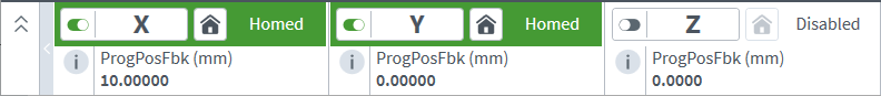
results = connected_controller.runtime.data_collection.get_results(data_config, num_points)

For this script, nothing is returned. However, in Automation1 Studio, as seen in figure 1 below, the X axis has moved to position 10, as commanded.

**Figure 1.** A screenshot of the Axis Dashboard from the Automation1 Studio application.

Extract and Plot Data

Any individual signal can be accessed from the results object. The expansive network of Python data analysis tools are now at a user’s disposal. For example, the matplotlib module can be used to plot the collected data.

#Storing the position command, feedback, and error signals collected from the controller into separate numpy arrays
pos_com = np.array(results.axis.get(a1.AxisDataSignal.PositionCommand, 'X').points)
pos_fbk = np.array(results.axis.get(a1.AxisDataSignal.PositionFeedback, 'X').points)
pos_err = np.array(results.axis.get(a1.AxisDataSignal.PositionError, 'X').points)

#Storing the time array collected from the controller
time_array = np.array(results.system.get(a1.SystemDataSignal.DataCollectionSampleTime).points)
time_array -=time_array[0]
time_array *=0.001
#Plotting the position command and feedback
figure_size = (40, 20)
plt.figure(1, figsize = figure_size)
font_size = 30
tick_size = 18
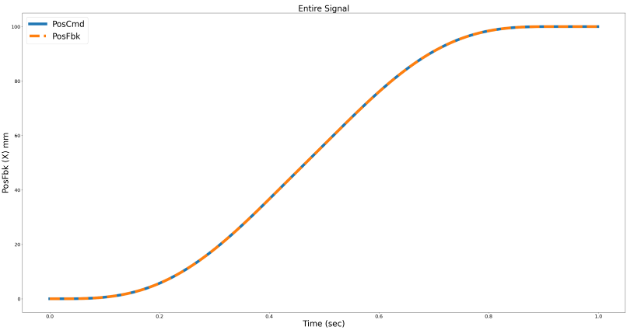
plt.plot(time_array, pos_com, linewidth = 10, label = 'PosCmd')
plt.plot(time_array, pos_fbk, linewidth = 10, linestyle = '--', label = 'PosFbk')
plt.xlabel('Time (sec)', fontsize = font_size)
plt.ylabel('PosFbk (X) mm',fontsize = font_size)
plt.title('Entire Signal',fontsize = font_size)

plt.xticks(fontsize = tick_size)
plt.yticks(fontsize = tick_size)
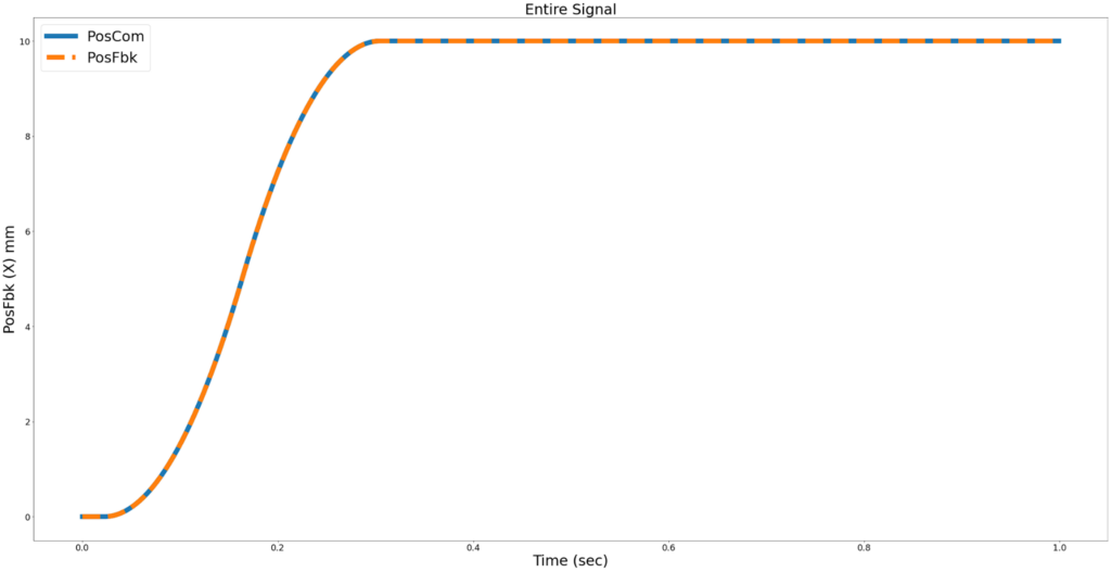
plt.legend(fontsize = font_size)

For this script, the following plot (figure 2) is collected. Because this command was run on a virtual (not real) axis of motion, the position feedback (PosFbk) matches the position command (PosCmd) perfectly.

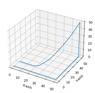
**Figure 2.** A graph using matplotlib’s Pyplot interface. To create this graph, a move is commanded to the Automation1 controller’s X axis. The position command and position feedback are captured over time, and the data signals are shown on this graph.

Additionally, you are able to plot 3D graphs using matplotlib in order to show movement in three dimensions. An example of such a graph is shown below:

#Configure data collection frequency and points
num_points = 10000
frequency = a1.DataCollectionFrequency.Frequency1kHz

data_config = a1.DataCollectionConfiguration(num_points, frequency)

#Adding the following signals to be collected on the x-axis
data_config.axis.add(a1.AxisDataSignal.PositionCommand, 'X')
data_config.axis.add(a1.AxisDataSignal.PositionFeedback, 'X')
data_config.axis.add(a1.AxisDataSignal.PositionError, 'X')

#Adding the time signal from the controller.
data_config.system.add(a1.SystemDataSignal.DataCollectionSampleTime)

#Adding the following signals to be collected on the y-axis
data_config.axis.add(a1.AxisDataSignal.PositionCommand, 'Y')
data_config.axis.add(a1.AxisDataSignal.PositionFeedback, 'Y')
data_config.axis.add(a1.AxisDataSignal.PositionError, 'Y')

#Adding the following signals to be collected on the z-axis
data_config.axis.add(a1.AxisDataSignal.PositionCommand, 'Z')
data_config.axis.add(a1.AxisDataSignal.PositionFeedback, 'Z')
data_config.axis.add(a1.AxisDataSignal.PositionError, 'Z')

#Enable and home the 'X' , 'Y' , and 'Z' axes
connected_controller.runtime.commands.motion.enable(['X','Y','Z'])
connected_controller.runtime.commands.motion.home(['X','Y','Z'])

#Data collection starts before the move 
connected_controller.runtime.data_collection.start(a1.DataCollectionMode.Snapshot, data_config)

#Linear move of 10 mm at 200 mm/s on the x-axis
connected_controller.runtime.commands.motion.movelinear('X', [50], 200)
connected_controller.runtime.commands.motion.movelinear('Y', [50], 200)
connected_controller.runtime.commands.motion.movelinear('Z', [50], 200)
connected_controller.runtime.commands.motion.moveabsolute(['X','Y','Z'], [5,5,5], [200,200,200])

#Return data after the move has been completed. 
results = connected_controller.runtime.data_collection.get_results(data_config, num_points)

x= np.array(results.axis.get(a1.AxisDataSignal.PositionCommand, 'X').points)
y= np.array(results.axis.get(a1.AxisDataSignal.PositionCommand, 'Y').points)
z= np.array(results.axis.get(a1.AxisDataSignal.PositionCommand, 'Z').points)
figure = plt.figure()
axis = figure.add_subplot(111, projection = '3d')

plt.plot(x, y,z)

axis.set_xlabel('X-axis')
axis.set_ylabel('Y-axis')
axis.set_zlabel('Z-axis')

plt.show()

For this script, the following three dimensional plot (figure 3) is displayed in the Jupyter notebook.

**Figure 3.** A three dimensional graph using matplotlib’s Pyplot interface. To create this graph, moves are commanded to the Automation1 controller’s X, Y and Z axes. The position commands are captured over time and the three dimensional positions are plotted in space, including a line tracing the points, in order, through space.

Note: Motion can be commanded directly from the API, but it can also be commanded by running a pre-scripted motion program. The API call for a compiled AeroScript program that already exists on the controller file system looks like this:

connected_controller.runtime.tasks[int Task].program.run("Program_Name.a1exe")

Please see About the Python API for more information.

Develop A Simple User Interface

Jupyter Notebook and ipywidgets (an open-source tool available to Python users) can be leveraged to develop a simple front end for data collection scripts. Similar to the libraries imported above, the ipywidgets library needs to be installed on a PC or workstation. A textbox widget can be created to prompt a user to input the desired step size. Next, a button widget can be created to perform the appropriately sized step and plot the results. The rest of the code in this paper can then be placed in a function that runs when the button is clicked.

Users can adjust the step size via the text box and move the stage via the button. A plot of the step can then be output without the user needing to write any additional code. In other words , a user interface can be created.


import ipywidgets as widgets

#Create a textbox widget
text_widget = widgets.FloatText(description = 'Step Size:', value = 10)

#Create a button widget
button_widget = widgets.Button(description = 'Run')

#Display widgets
display(text_widget, button_widget)

#Function to step and plot the results
def button_function(b):
    print('Stepping...')
    
    connected_controller = a1.Controller.connect()
    connected_controller.start()
    
    connected_controller.runtime.commands.motion_setup.setupcoordinatedspeed(200)
    axis = ['X', 'Y']
    connected_controller.runtime.commands.motion.enable(axis)
    connected_controller.runtime.commands.motion.home(axis)
    
    num_points = 1000
    frequency = a1.DataCollectionFrequency.Frequency1kHz

    data_config = a1.DataCollectionConfiguration(num_points, frequency)

    #Adding the following signals to be collected on the x-axis
    data_config.axis.add(a1.AxisDataSignal.PositionCommand, 'X')
    data_config.axis.add(a1.AxisDataSignal.PositionFeedback, 'X')
    data_config.axis.add(a1.AxisDataSignal.PositionError, 'X')

    #Adding the time signal from the controller to be connected.
    data_config.system.add(a1.SystemDataSignal.DataCollectionSampleTime)
    
    #Enable and home the 'X' and 'Y' axes
    connected_controller.runtime.commands.motion.enable(['X','Y'])
    connected_controller.runtime.commands.motion.home(['X','Y'])
    
    #Data collection starts before the move 
    connected_controller.runtime.data_collection.start(a1.DataCollectionMode.Snapshot, data_config)

    #Linear move on x-axis at 200 mm/s, distance is what is typed into text_widget
    connected_controller.runtime.commands.motion.movelinear('X', [text_widget.value], 200)

    #Return data after the move has been completed. 
    results = connected_controller.runtime.data_collection.get_results(data_config, num_points)

    #Storing the position command, feedback, and error signals collected from the controller into separate numpy arrays
    pos_com = np.array(results.axis.get(a1.AxisDataSignal.PositionCommand, 'X').points)
    pos_fbk = np.array(results.axis.get(a1.AxisDataSignal.PositionFeedback, 'X').points)
    pos_err = np.array(results.axis.get(a1.AxisDataSignal.PositionError, 'X').points)

    #Storing the time array collected from the controller
    time_array = np.array(results.system.get(a1.SystemDataSignal.DataCollectionSampleTime).points)
    time_array -=time_array[0]
    time_array *=0.001

    #Plotting the position command and feedback
    figure_size = (40, 20)
    plt.figure(1, figsize = figure_size)

    font_size = 30
    tick_size = 18

    plt.plot(time_array, pos_com, linewidth = 10, label = 'PosCmd')
    plt.plot(time_array, pos_fbk, linewidth = 10, linestyle = '--', label = 'PosFbk')

    plt.xlabel('Time (sec)', fontsize = font_size)
    plt.ylabel('PosFbk (X) mm',fontsize = font_size)
    plt.title('Entire Signal',fontsize = font_size)

    plt.xticks(fontsize = tick_size)
    plt.yticks(fontsize = tick_size)

    plt.legend(fontsize = font_size)
    
#When button_widget is clicked, run button_function

button_widget.on_click(button_function)

For this script, the following user interface (figure 4) is displayed:

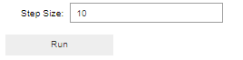
**Figure 4.** A simple user interface is created in Jupyter notebook.

Entering a number (in this case 10) and clicking “run” generates the following (figure 5) in the Jupyter notebook:

**Figure 5.** A graph using matplotlib’s Pyplot interface. To create this graph, use the simple user interface shown in figure 4. The position command and position feedback of the X axis are captured over time, and the data signals are displayed on this graph.

Summary

The Python API for Automation1 is an extremely powerful tool for integrating Python data analysis with Automation1 data collection. It can be used to move stages, quickly process data and develop graphical user interfaces. Users can leverage the flexible API to quickly create programs and tools for their own processes.

Consultation

Buy Now

Can you have it all when producing displays?

Display Week 2024