Capability Overview, Electronics, Laser Scan Heads, Laser Systems
Capability Overview
Using the Galvo Calibration File Converter with the Automation1-GL4
Calibrating the field of view for scanners is typically an iterative process where a series of marks are placed on a substrate and the location of these marks is used to create a calibration file. The process is repeated until final system accuracy is reached. Each iteration of the mark and measure sequence must combine the new measurement values with the current calibration table to create a new calibration table that incorporates the new correction adjustments. When the tables are of the same resolution, the values can be added directly to each other. When the density of the marks in the tables to be combined is not equal, an algorithm must be applied to interpolate lower resolution data with higher resolution data.
Aerotech’s Galvo Calibration File Converter (GCFC) application can be used to merge measurement data and existing calibration files during the calibration process. The densities of the tables to be merged do not have to match because GCFC will interpolate the correction values of the lower density table to match those of the higher density table.
This document will outline the procedures required to create new correction tables from real error measurements and merge existing correction tables for Aerotech’s laser scan head drive, the Automation1 GL4.
Calibration File Creation
When creating tables through a manual measurement procedure, users will typically start by marking a low density grid (such as 3 x 3), measuring the placement accuracy of each location in the grid and then applying the measurements in a correction table on the controller. Next, they activate the correction table on the controller and mark a second grid at an increased density (such as 5 x 5). This sequence is repeated until the desired results are attained over the entire working area of the scanner.
For applications where the measurement of marked grids is automated, the grid spacing can start at a much higher density (such as 33 x 33) since the process does not require manual measurement of the placement error at each location in the grid.
Manual File Creation Process
Step 1: Create a New File
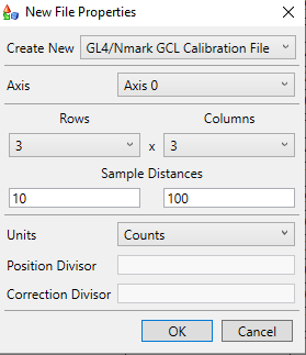
To create a new file, select New from the File menu. A Calibration File Type dialog will appear (Figure 1). Descriptions of the field settings within the dialog are listed below:
- Create New: Select GL4 Calibration File.
- Axis: The axis index of the first axis on the Automation1-GL4. Note: the axis index is found in Automation1 Studio’s Configure Workspace by opening the Manage Axes window.
- Sample Distance: Distance between grid points. Distance is scaled by the “Position Divisor.”
- Units: Set the unit type for the correction values that will be entered in the table; this is typically set to Primary Units to reflect the user programming units. Note: Set to Primary Units for all Automation1 controller configurations.
- Position Divisor: Optional scaling of the sample distance value relative to the Primary Units. If this field is set to 1000 and the Primary Units are set to “mm” in Automation1, then the sample distance is specified in microns. If no value is given, then the sample distance is defined by the specified unit type.
- Correction Divisor: Optional scaling of correction units relative to the primary units. If this value is set to 1000 and the Primary Units are “mm,” then the correction values are entered in microns. If no value is given, then the correction values are defined by the specified units type.
The GCFC application is not aware of the scanner’s field of view size. The Sample Distance and the Grid Size settings must be chosen such that the resulting table matches the scanner’s field of view.
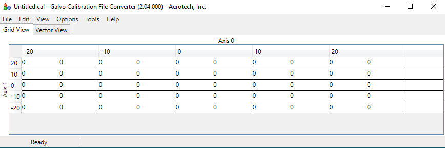
Entering the data and clicking the OK button creates a blank correction file (Figure 2). Figure 2 shows a 5 x 5 table with a sample distance of 10. Note that Axis 1 values increase left to right, and Axis 0 values increase bottom to top. If desired, axes can be swapped and the positive move direction of each axis can be inverted via the Change Field of View Orientation menu item in the View dropdown menu.
Step 2: Enter Correction Table Elements
By default, the table elements are assumed to be corrections. This is a value that is added to the commanded position to arrive at the desired position.
Positionmodified = Positioncommand + CorrectionValue
The values can also be entered/displayed as errors. This value is subtracted from the commanded position to arrive at the desired position.
Positionmodified = Positioncommand – Error
Setting the values to show as corrections or errors is done through the Show Values As menu item on the View menu.
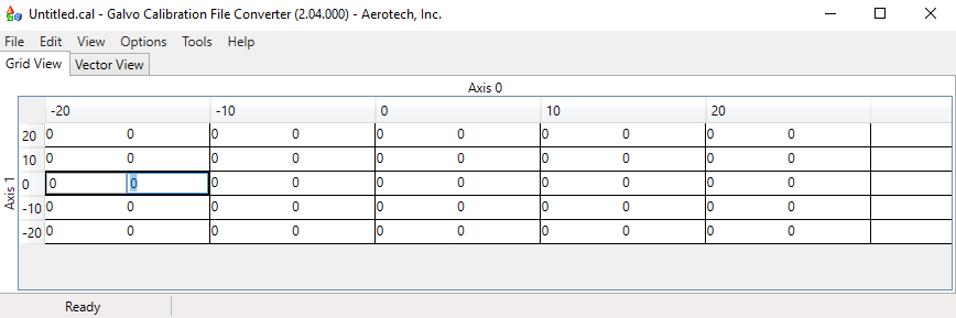
Once the correction field type is specified, a user enters the values into the table by double‐clicking on the desired table element and typing in a value (Figure 3).
As an alternative to manually entering correction information, the data can be stored in a Comma Separated Values (CSV) file and imported by GCFC. See the Automated Calibration section at the end of this discussion for information on the CSV file format.
Step 3: Creating and Activating a Correction File
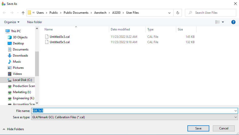
To create a calibration file from the entered data, select the Save As menu item from the File menu, set the type as GL4 Calibration Files (*.cal) and enter in a file name (Figure 4). For this example, the results are saved in a file called “5×5.CAL.”
Automation1 stores all 2D calibration tables in a single file. If the Automation1-GL4 is the only active 2D calibration table, then the controller can be configured to load the calibration file created by the GCFC. If more than one 2D table is contained within the CAL file – for example, 2D calibration of X/Y stages or there is more than one Automation1-GL4 – then the contents of the file created in this step must be copied directly into the master 2D CAL file.
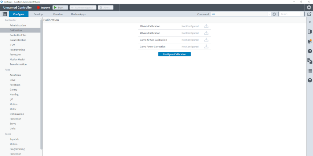
The 2D calibration file is set up in the Configure Workspace as shown in Figure 5.
The Automation1 controller must be reset and the Automation1-GL4 axis homed to activate the contents of the calibration file.
Step 4: Merging Calibration Files
After the calibration file has been activated, users measure the resulting accuracy and repeat steps 1 through 3 to create a new calibration file based on the measured results. Then they save this file under a new name. The new calibration file does not have to be the same size as the previously created file.
To combine the active calibration file with the new measured calibration data, select the Merge option from the File menu and browse for the name of the file that contains the calibration data that is currently active on the controller (in this example, the file name is “5×5.CAL”). If the calibration table’s contents are copied into a master 2D calibration file, it’s important to select the file from which the table was copied and not the master calibration file. GCFC will display the results of the merged tables, and then the user can save and activate the contents as outlined in Step 3.
Step 5: Repeat Steps 1‐4 as Required
For a given grid size, the measured accuracy should converge after 2‐3 iterations of the mark and measure sequence, as outlined above.
Automated Calibration Process
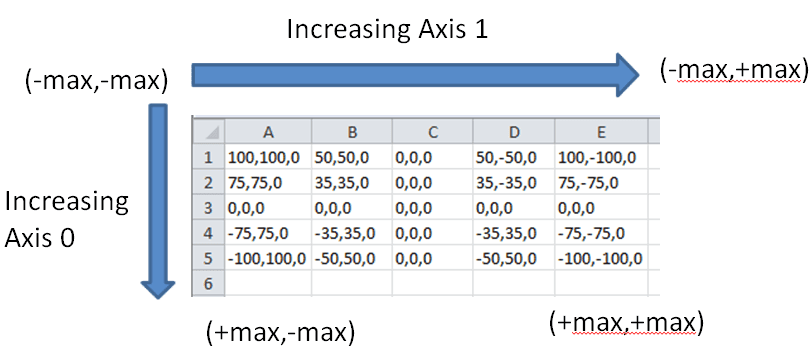
The GCFC can import CSV files that contain the measurement process results. For example, a vision process can acquire the marks made by the scanner on the substrate, measure the placement accuracy and store the results directly into a CSV file. The order of the correction elements in the CSV file differs from the Grid View because Axis 0 positions increase top to bottom and Axis 1 positions increase left to right (Figure 6).
When a CSV file is opened, the user must specify the “Calibration File Type” data (Figure 7). See Step 1 for a description of the input data.
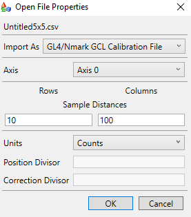
Once the CSV file is opened, the data can be saved as a 2D calibration file using the Save As option of the File menu with the file type set as “cal” (as outlined in Step 3).
Alternatively, the measurement process can create an Aerotech compatible 2D calibration file format directly. The 2D calibration file can be read by GCFC and merged with an existing 2D calibration file on the hard drive. Working with 2D calibration files eliminates the need to specify axis information, grid size and correction scaling information when using the CSV import approach as this information will be written in the 2D calibration file by the measurement process.